
A normal distribution is one of the most famous statistics distributions and it is informally called bell curve shape. Normal distributions are important in statistics and are often used in the natural and social sciences to represent real-valued random variables whose distributions are not known. Especially a normal standard distribution is frequently seen in probability distiribution where the mean value equals to 0 and the standard deviation equals to 1. It is fundamental characteristic that is used under the central limit theorem.
It states that, under some conditions, the average of many samples (observations) of a random variable with finite mean and variance is itself a random variable—whose distribution converges to a normal distribution as the number of samples increases.
Normal Distribution
Here’s a good reference to understand the normal distribution with Python code. After I learned the normal distribution and characteristics, I wondered how we could know a distribtion conforms to the normal distribution. In this guide, I will show the result of my research about how to do test of normality in Scipy library in Python for data.
Understanding the Normal Distribution (with Python)
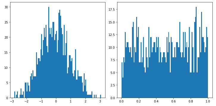
Let’s prepare 2 data sets, one is random data points following the normal distribution and one is purely random data points with Numpy library.
- Use probplot against quantiles of the normal distribution
- Use shapiro to perform the Shapiro-Wilk test for normality
- Calculate Skewness and kurtosis and compare the values
Use probplot against quantiles of the normal distribution
probplot calculates quantiles for a probability plot and generates a probability plot of sample data against the quantiles of a specified theoretical distribution. In default the normal distribution is configured for a theoretical distribution. The term “probability plot” sometimes refers specifically to a Q–Q plot, sometimes to a more general class of plots, and sometimes to the less commonly used P–P plot.
Probability prot or a Q-Q plot (quantile-quantile plot) can be used to compare two probability distributions by plotting the quantiles against each other. But in this case we use a probability plot to compare a data set to a theoretical model that is the normal distribution. The function draws the theoretical distribution in x axis and calculate quantiles and draws it in y axis like below.

You might notice 45% red line in both figures. What is it? If the ordered values are similar to the theoretical quantiles then, the points in the Q–Q plot will approximately lie on the red line. In another situation, if the data and the distribution are linearly related, the points in plot will approximately lie on a line, but not necessarily on the red 45% line.
The left figure shows data in y axis was almost similar to the normal distribution and it is. However the right figure explains the random data doesn’t follow the normal distribution at all. Interpreting the probability plot is not easy, if you look at y axis in the right figure the scale between 0.0 to 1.0 would be a clue how these quantiles were drawn.
Use shapiro to perform the Shapiro-Wilk test for normality
What is the Shapiro-Wilk test? In one word, the Shapiro-Wilk test tests the null hypothesis that the data was drawn from a normal distribution specifically. By using shapiro you will need to care about 2 variables, statistic and pvalue. Here’s the W statistic explanation.
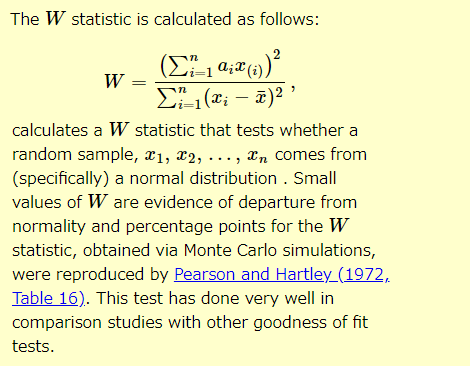
For N > 5000 the W test statistic is accurate but the p-value may not be. The chance of rejecting the null hypothesis when it is true is close to 5% regardless of sample size. This means p-value is around 0.05 or above 0.05, we can’t reject this null hypothesis. So this is possibly normally distributed. If p-value is far from 5% (0.05) then we can reject the null hypothesis. Let’s see how the calculation went for our data.
The Shapiro-Wilk test gave the same result, the first data set is likely the normal distribution while the second random data showed quite low p-value, which means that we can reject the null hypothesis.
Calculate Skewness and kurtosis and compare the values
The last one looks little tricky. This is the method to check skewness and kurtosis statistics and compare to the normal distribution’s values. Because these 2 statistics are telling us about the shape of the distribution, the characteristics of the shape. This is not actually the test of normality but give more insights about the distribution’s shape for some degree.
Skewness is a measure of the symmetry in a distribution. A symmetrical dataset will have a skewness equal to 0. So, a normal distribution will have a skewness of 0.
Kurtosis is a measure of the combined sizes of the two tails. It measures the amount of probability in the tails. The value is often compared to the kurtosis of the normal distribution, which is equal to 3.
Are the Skewness and Kurtosis Useful Statistics?
stats.skew and stats.kurtosis are the built-in functions you can compute statistics easily. In default stats.kurtosis is set to Fisher’s definition use. If Fisher’s definition is used, then 3.0 is subtracted from the result to give 0.0 for a normal distribution. I changed it to using Pearson’s definition, so the value 3 should appear for data set close to the normal distribution.
Here’s the sample code in Scipy.
If a skewness is positive, it means the right hand tail is more longer and if a skewness is negative, the left hand tail tends to be longer in general. If it falls between -0.5 and 0.5, that data are fairly symmetrical.
A kurtosis is said to measure the tail heaviness of the distribution. It increases as the tails become heavier while it decreases when the tails get lighter. We can assume that a kurtosis is 3 for the normal distribution.
For the 2 data sets, the first one has the close statistics values for the normal distribution. Please note that skewness and kurtosis are the statistics not to test the normality but we can just compare statistics values to know if a given distribution has closer values.